Understanding the SIR model

Introduction

In class we covered the SIR model with births and deaths. As a quick refresher: susceptible individuals (\(S\)) become infected and move into the infected class (\(I\)), and then infected individuals who recover move into the recovored, or immune, class (\(R\)). Assuming the birth rate is equal to the death rate (\(\mu\)) gives:

\[\begin{align*} \frac{dS}{dt} &= \mu N -\beta S I - \mu S\\ \frac{dI}{dt} &= \beta S I - \gamma I - \mu I\\ \frac{dR}{dt} &= \gamma I - \mu R. \end{align*}\]

So what do these terms mean? Suppose the unit of time we are considering is days, then

• \(\mu N\) represents the number of births into the population per day (we assume everyone is born susceptible)
• \(\beta S I\) represents the number of susceptible individuals that become infected per day
• \(\mu S\) (or \(\mu I\)/ \(\mu R\)) is the number of susceptible (or infected/ immune) individuals that die per day.
• \(\gamma I\) is the number of infected individuals that recover per day.

From these equations we can create a flow diagram showing the direction of movement of individuals through these compartments:

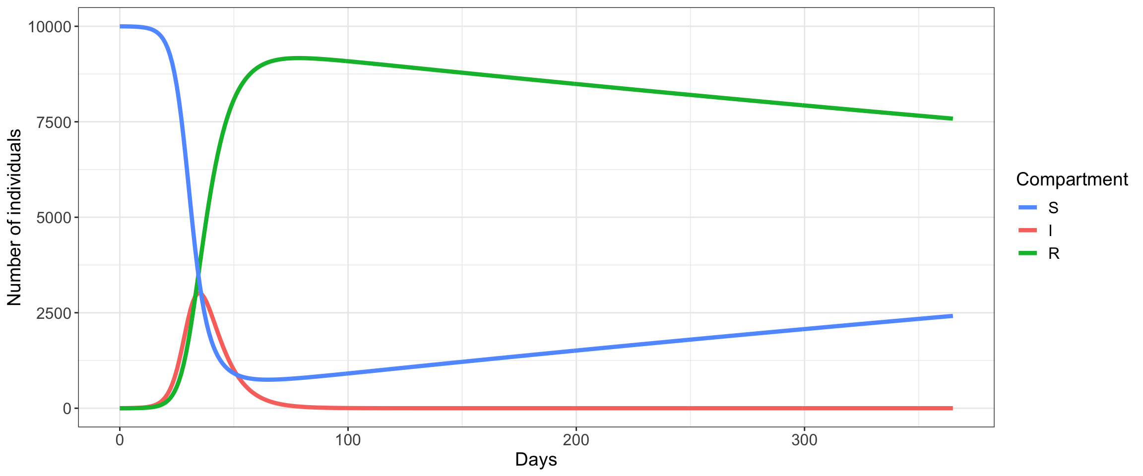
To find the number of susceptible, infected, and recovered individuals over time, we have to solve these equations using numerical integration methods. In this class we will use R to do this. Here’s an example of what the outcome of solving these equations looks like for a given set of parameters (\(\beta = 4 \times 10^{-5}, \mu = 7 \times 10^{-4}, \gamma = 1/7\); note: this corresponds to an \(R_0\) of about 3).

Incorporating vaccination

To incorporate vaccination we need to modify the equations above so that a proportion, \(p\) say, of the new births into the population are vaccinated (and thus immune to infection). Those that are vaccinated will avoid the susceptible class and go straight to the recovered class, whereas those that are unvaccinated will go into the susceptible class as before.

If \(p\) is the proportion vaccinated, then \(1 - p\) is the proportion left unvaccinated. Therefore the number of new births that are vaccinated (per unit time) is \(\mu N p\), and the number unvaccinated is \(\mu N (1 - p)\).

Our equations therefore become:

\[\begin{align*} \frac{dS}{dt} &= \mu N (1 - p) -\beta S I - \mu S\\ \frac{dI}{dt} &= \beta S I - \gamma I - \mu I\\ \frac{dR}{dt} &= \gamma I - \mu R + \mu N p. \end{align*}\]

And our flow diagram now looks something like this:

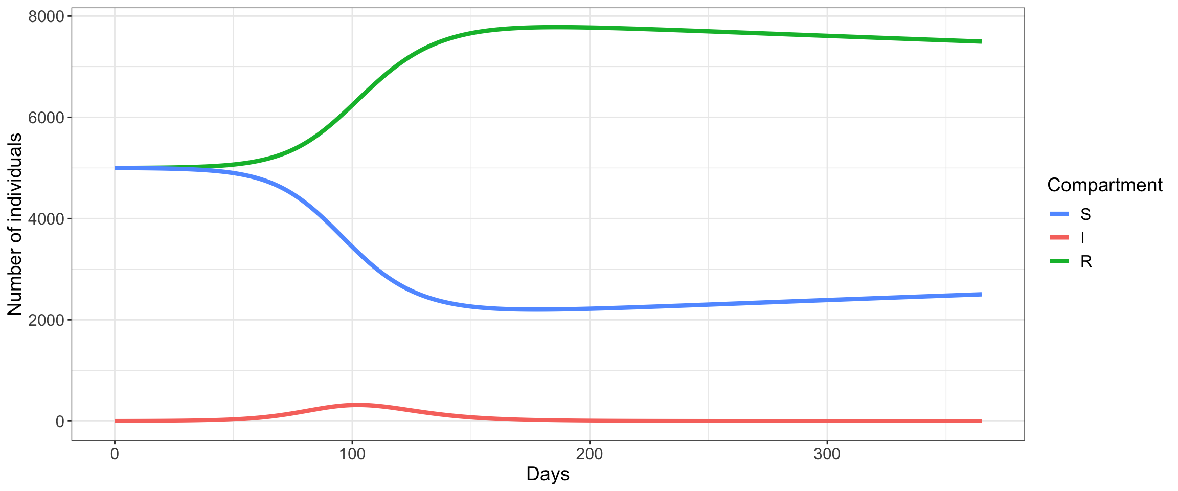
Here’s the outcome of solving these equations with \(p = 0.5\) (and all other parameters as before). Note: now the effective reproduction number is \(R_0 \times (1 - p) \sim 3 \times 0.5 = 1.5\).

In the interactive plot below you can explore what happens to the outcome as you change different model parameters, e.g:

• how does changing \(R_0\) impact the shape of the epidemic curve?
• what happens when you add in births/ deaths (i.e. change \(\mu = 0\) to \(\mu \geq 0\))?
• what happens when you include vaccination?

To create your own interactive plots in R, like the one above, check out my R package shinySIR