SIS model for malaria

Jan 17, 2018 7 min read R

Background: simple SIS model

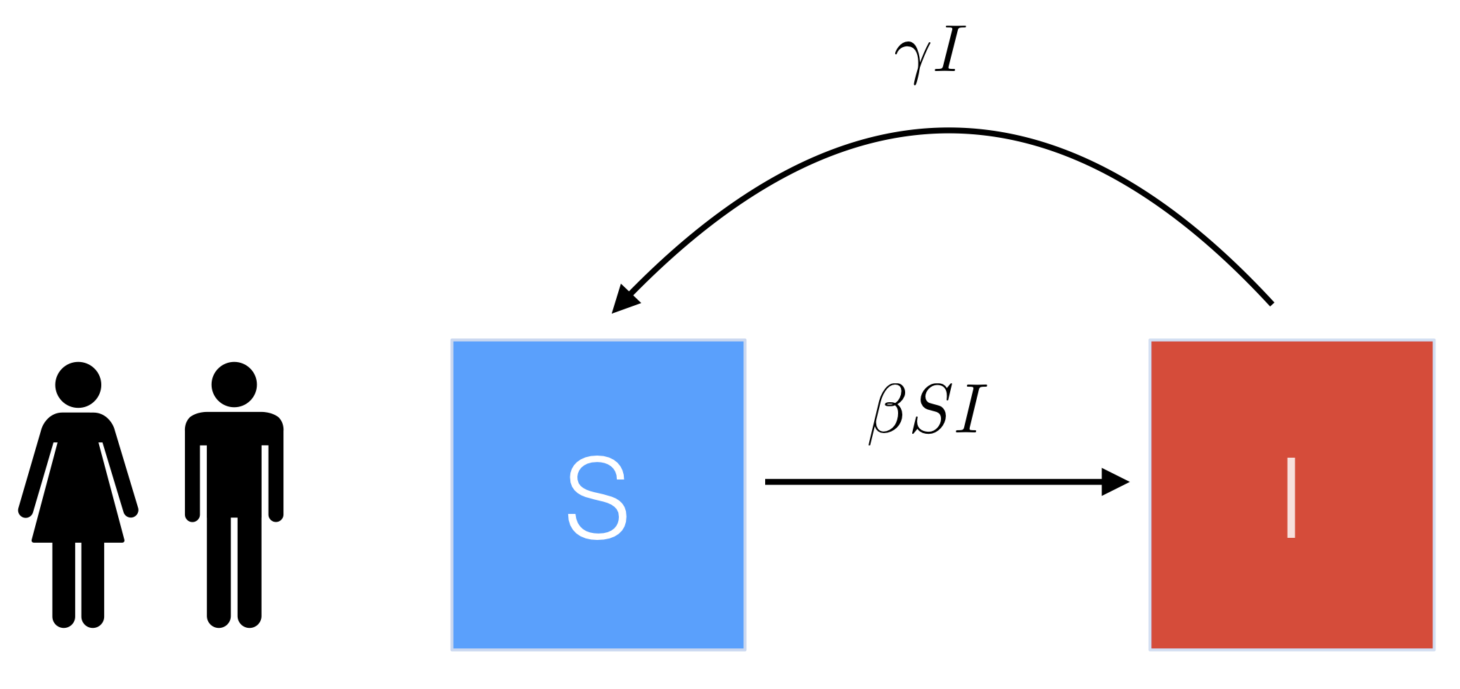
Let’s start by refreshing the basics of the SIS model. Susceptible individuals ($S$) become infected and move into the infected class ($I$), and then infected individuals who recover move straight back to the susceptible class (so there’s no period of immunity like in the SIR model). For simplicity we will ignore births and death, and also use a proportional model i.e. $S$ + $I$ = $N$ = 1. The basic flow diagram is shown below.

An example simulation of this model is shown in Figure 1, and the corresponding equations are

\[\begin{align*} \frac{dS}{dt} &= - \beta S I + \gamma I\\ \frac{dI}{dt} &= \beta S I - \gamma I. \end{align*}\]

$Example simulation of the simple SIS model with $\gamma = 7$ day$^{-1}$, $R_0 = 3$ and $\beta = R_0\times \gamma$.$

Figure 1: Example simulation of the simple SIS model with $\gamma = 7$ day$^{-1}$, $R_0 = 3$ and $\beta = R_0\times \gamma$.

If we focus on just the $I$ equation, then we can eliminate $S$ by using the fact that $S + I = 1 \Rightarrow S = 1 - I$. So

\[\begin{align} \frac{dI}{dt} &= \beta S I - \gamma I \nonumber\\ \Rightarrow ~~~ \frac{dI}{dt} & = \beta (1 - I) I - \gamma I\label{eqn:SIS}. \end{align}\]

This will makes things simpler when we come to calculating $R_0$ for the extended malaria model.

Transmission rate

In this simple SIS model, the effective transmission rate, $\beta$, can be thought of as the product of the number of contacts per individual (per unit time) and the probability that each of these independent contacts will result in infection i.e.

\[\begin{align*} \beta &= (\#~contacts~per~individual) \times (prob.~infection) \end{align*}\]

Incorporating human-mosquito interactions

To extend the simple SIS model above to malaria dynamics, we need to account for both human and mosquito populations in our model equations.

To do this, we define $S_h$ and $I_h$ to represent the proportion of humans that are susceptible and infected, respectively, and $S_m$/ $I_m$ to represent the proportion of mosquitos that are susceptible/ infected. A basic flow diagram is shown below.

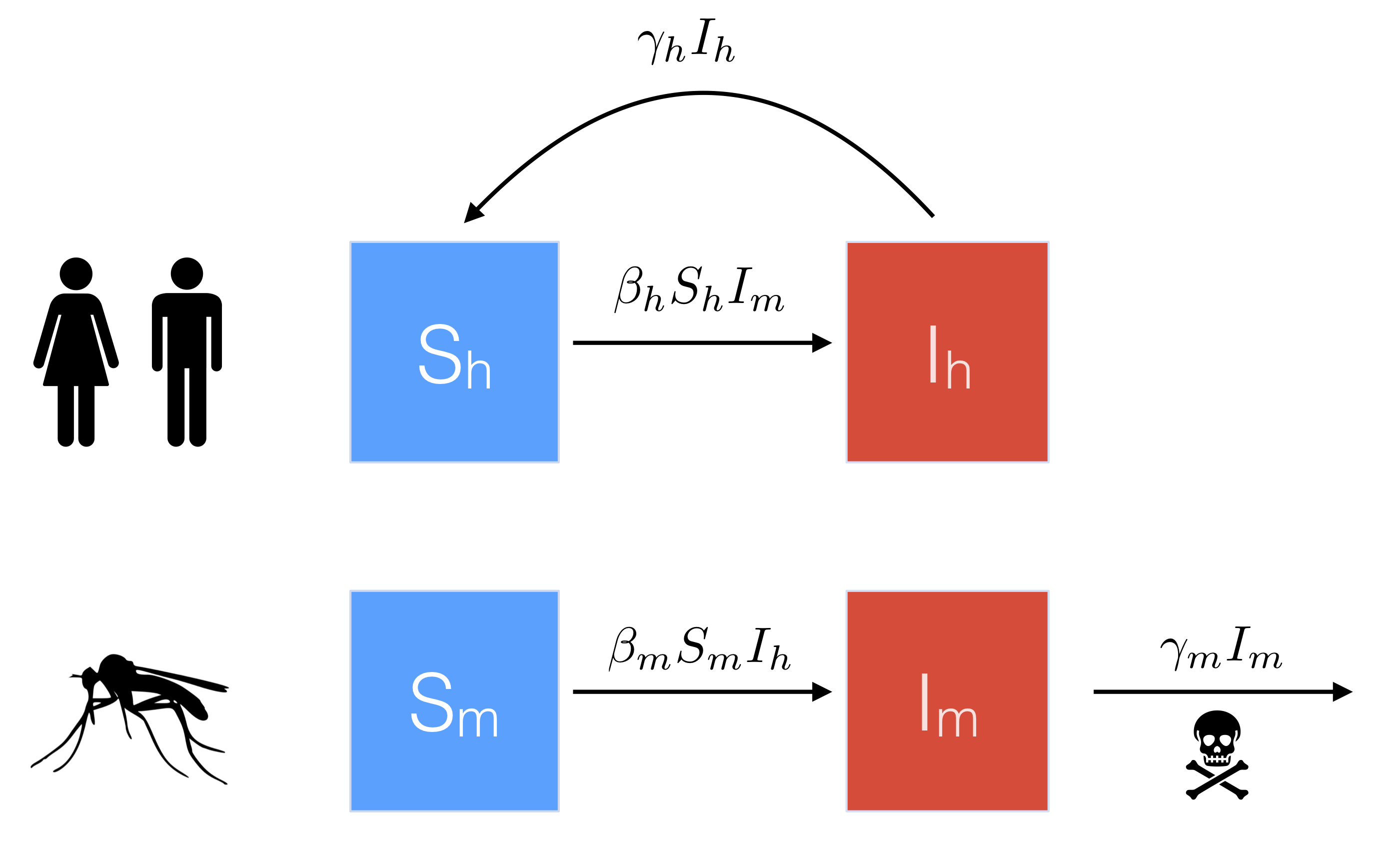
$Note that in contrast to the human population, which recover at rate \gamma_h, we assume that mosquitos do not recover from disease, and instead die at rate \gamma_m.$

Note that in contrast to the human population, which recover at rate $\gamma_h$, we assume that mosquitos do not recover from disease, and instead die at rate $\gamma_m$.

Similar to the simple SIS model, we assume $S_h = 1 - I_h$, and $S_m = 1 - I_m$. We can then modify our equation for $dI/dt$ above to describe the proportion infected in both the human and mosquito populations.

Humans

First, for infected humans, we know that each new infected case can only arise when a susceptible human ($S_h = 1 - I_h$) comes into contact (i.e. is bitten) by an infected mosquito ($I_m$). Therefore,

\[\begin{align*} \frac{dI_h}{dt} & = \beta_h (1 - I_h) I_m - \gamma_h I_h, \end{align*}\]

where $\beta_h$ is the effective transmission rate of humans being infected by mosquitos. Similar to the simple SIS model above, we can think of $\beta_h$ as the product of the number of mosquito contacts (i.e. bites) per human (per unit time) and the probability that each independent bite will result in infection i.e.

\[\begin{align*} \beta_h &= (\#~contacts~per~human) \times (prob.~infection~from~mosquito)\\ & = ~~~(\#~bites~per~human) ~~\times (prob.~infection~from~mosquito). \end{align*}\] At this stage, notice that we can express the $\# ~bites ~per ~human$ as \[\begin{align*} (\#~bites~per~human) ~ &= ~(\# ~bites ~per ~mosquito) ~\times ~(\# ~mosquitos ~per ~human) \end{align*}\]

(To think about this intuitively, from the perspective of a susceptible human, we would expect the number of times they are bitten to increase if there are (1) more mosquitos around AND (2) if the mosquitos around are biting more frequently.) This means that we can then write

\[\begin{align} \beta_h& = (\#~bites~per~mosquito) \times (\#~mosquitos~per~human) \times (prob.~infection~from~mosquito)\nonumber\\ & = ~~~~~~a ~~~~~~\times~~~~~~ m ~~~~~~\times ~~~~~~b\label{eqn:bites}. \end{align}\]

Mosquitos

Similarly, for infected mosquitos, we know that each new infected case can only arise when a susceptible mosquito ($S_m = 1 - I_m$) comes into contact (i.e. bites) an infected human ($I_h$). Therefore,

\[\begin{align*} \frac{dI_m}{dt} & = \beta_m (1 - I_m) I_h - \gamma_m I_m, \end{align*}\]

where $\beta_m$ is the effective transmission rate of mosquitos being infected by humans. Similar to above, we can think of $\beta_m$ as the product of the number of human contacts (i.e. bites) per mosquito (per unit time) and the probability that each independent bite will result in infection i.e.

\[\begin{align*} \beta_m &= (\#~contacts~per~mosquito) \times (prob.~infection~from~human)\\ & = ~~~(\#~bites~per~mosquito) ~~~\times (prob.~infection~from~human). \end{align*}\]

Notice that this expression is slighty simpler than the earlier expression for $\beta_h$, since we already know the # bites per mosquito (it’s just equal to $a$ as we defined in equation ()!). Therefore,

\[\begin{align} \beta_m & = (\#~bites~per~mosquito) \times (prob.~infection~from~human)\nonumber\\ & = ~~~~~~a ~~~~~~\times~~~~~~c. \end{align}\]

Combining equations

Substituting $\beta_h = amb$ and $\beta_m = ac$ into our differential equations then gives the extended SIS model for malaria transmission between humans and mosquitos:

\[\begin{align*} \frac{dI_h}{dt} & = amb (1 - I_h) I_m - \gamma_h I_h\\ \frac{dI_m}{dt} & = ac (1 - I_m) I_h - \gamma_m I_m. \end{align*}\]

An example simulation of these equations is shown in Figure 2.

$Example simulation of the SIS malaria model with $\gamma_h = 7$ day$^{-1}$, $\gamma_m = 3$ day$^{-1}$, $m = 2, a = 4, b = 0.05$, and $c = 0.09$ (so again $R_0 \sim 3$).$

Figure 2: Example simulation of the SIS malaria model with $\gamma_h = 7$ day$^{-1}$, $\gamma_m = 3$ day$^{-1}$, $m = 2, a = 4, b = 0.05$, and $c = 0.09$ (so again $R_0 \sim 3$).

Finding $R_0$

To find $R_0$ we want to focus on the human population (i.e. we want to know how many secondary human infections are likely to occur). Doing this requires making some simplifying assumptions about the mosquito population.

Specifically, for this class, we will assume that the mosquito dynamics are already at equilibrium (i.e. $dI_m/dt = 0$). As an example, this could represent the case where malaria is endemic in the mosquito population and we want to know what will happen when an epidemic is introduced into a new naive human population.

So the steps we will take are:

Set $dI_m/dt = 0$ and solve to find an expression for the proportion of infected mosquitos, $I_m$, at this endemic point;
Look at what happens to the proportion of infected humans at the beginning of the epidemic i.e. set $dI_h/dt > 0$ (this is just like we’ve done previously e.g. with the SIR model).

1. Finding the proportion of infected mosquitos

Setting $dI_m/dt = 0$ and expanding out the brackets gives

\[\begin{align*} ac (1 - I_m) I_h - \gamma_m I_m & = 0,\\ ac I_h - ac I_m I_h - \gamma_m I_m & = 0. \end{align*}\] Then isolating all terms containing $I_m$ on one side, we get \[\begin{align*} ac I_m I_h + \gamma_m I_m & = ac I_h\\ I_m (ac I_h + \gamma_m) & = ac I_h\\ I_m & = \frac{ac I_h}{ac I_h + \gamma_m}.\\ \end{align*}\]

2. Considering the start of the human epidemic

Setting $dI_h/dt > 0$ and using the expression for $I_m$ that we just found gives \[\begin{align*} amb (1 - I_h) I_m - \gamma_h I_h & > 0,\\ amb (1 - I_h) \frac{ac I_h}{ac I_h + \gamma_m} - \gamma_h I_h & > 0. \end{align*}\]

Now, since we are at the start of the epidemic, we know that $S_h(0) = 1 - I_h(0) \sim 1$ (i.e. basically the entire population is suceptible), and so we can set $1 - I_h$ = 1 in the above equation to simplify things to

\[\begin{align*} amb \frac{ac I_h}{ac I_h + \gamma_m} - \gamma_h I_h & > 0,\\ amb \frac{ac}{ac I_h + \gamma_m} - \gamma_h & > 0,\\ \frac{ambac}{ac I_h + \gamma_m} & > \gamma_h. \\ \end{align*}\] Finally, rearranging the left hand side numerator and diving both sides by $\gamma_h$ gives \[\begin{align*} \frac{ma^2bc}{\gamma_h( ac I_h + \gamma_m)} & > 1. \end{align*}\]

Finally, we can simplify this one stage further by assuming that the initial proportion of infected humans is very small, or even zero, i.e. $I_h(0) \sim 0$. This means we can set $ac I_h = 0$, so that

\[\begin{align*} \frac{ma^2bc}{\gamma_h\gamma_m} & > 1. \end{align*}\]

Therefore our final expression for $R_0$ is

\[\begin{align*} R_0 = \frac{ma^2bc}{\gamma_h\gamma_m}. \end{align*}\]

SIS model Lectures

Sinead E. Morris

Influenza Modeling Consultant

I work at the intersection of mathematical modeling, epidemiology, and infectious diseases.